Poirot and the RNN murders

Imagine you’re in a warm, lively London pub in 1920, sharing a beer with some friends. Your attention first settles on a man at a nearby table, sipping a glass of crème de cassis—an unusual choice for such a busy spot. Then you notice his neatly trimmed mustache. You recognize Poirot, the famous Belgian detective !
He is speaking with someone who seems to be a witness to a troubling case. He takes down quick notes in a small notebook, capturing every snippet of conversation. Each word, building on the last, sparks a new idea in his mind, like puzzle pieces clicking into place.
That's pretty much how a Recurrent Neural Network, or RNN, works—it listens to every word in a sentence. It recalls what was said before to figure out what might come next.
Unlike Poirot, who undoubtedly noticed and remembered every detail of a conversation, RNNs struggle to retain information from much earlier in a sequence. This limitation led to further advances in deep learning and, ultimately, to the development of Transformers. Despite these shortcomings, RNNs remain a valuable tool for understanding large language models. They demonstrate how to process data in a specific order—such as words in a sentence —and serve as an intermediate step toward comprehending transformer-based networks, which rely on attention mechanisms.
In the following sections, you will explore the inner workings of a RNN, discovering the role of each component and gaining simplified insights into the underlying mathematics.
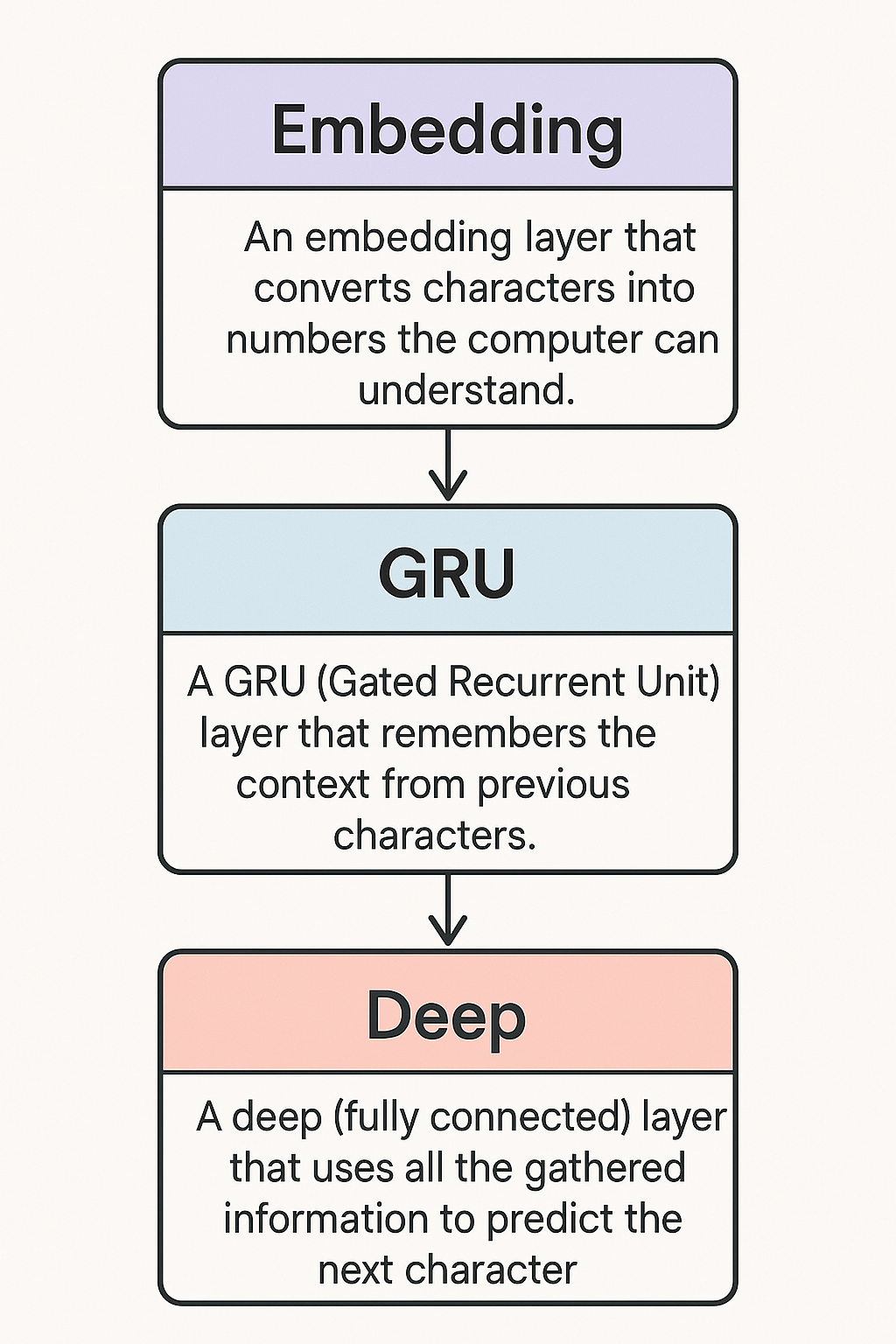
Let's see how to use an RNN to predict the next character in a provided sequence. To do it, we' will build a model with three layers, explaining what each layer does and how it contributes to the final result.
- First, an embedding layer converts characters into numerical representations that capture their semantic meaning.
- Next, a GRU (Gated Recurrent Unit) layer that remembers the context from previous characters.
- Finally, a deep (fully connected) layer that uses all the gathered information to predict the next character.
It is the brain, the little grey cells on which one must rely
One way to train our model is by breaking down a famous Poirot quote into overlapping segments using a sliding (moving) window. We pair each segment with the following segment, which serves as our target because it contains the subsequent character in the sequence. By comparing these pairs, the model learns to predict the next character and gradually develops an understanding of the text’s flow. Let's take an example to get a concrete understanding
- We start by taking a fixed chunk of 15 characters from the quote, for example: "It is the brain"
- Then, we slide the window one character forward, giving us: "t is the brain,
The result is visible in the table 1
| Input | Target |
| is the brain, t | s the brain, th |
| s the brain, th | the brain, tha |
Note that the second sequence is exactly the same as the first, but shifted by one character. In our setup, the model uses the first sequence (window) and sends it character by character through all its layers, attempting to predict the corresponding character at the same index in the second sequence. This process is repeated for the entire sequence, using every possible pair of shifted sequences.
Tokenisation
First we need to define a vocabulary of tokens in our text. In language modeling, the vocabulary is the set of all symbols or tokens that the model can recognize.
The vocabulary is not always composed of word —they could be subwords, characters, or even punctuation (e.g., "play", "##ing", ".", etc.). That will depend on the tokenizer we will use. Let's see the tokens for our sentence using OpenAI Tokenizer
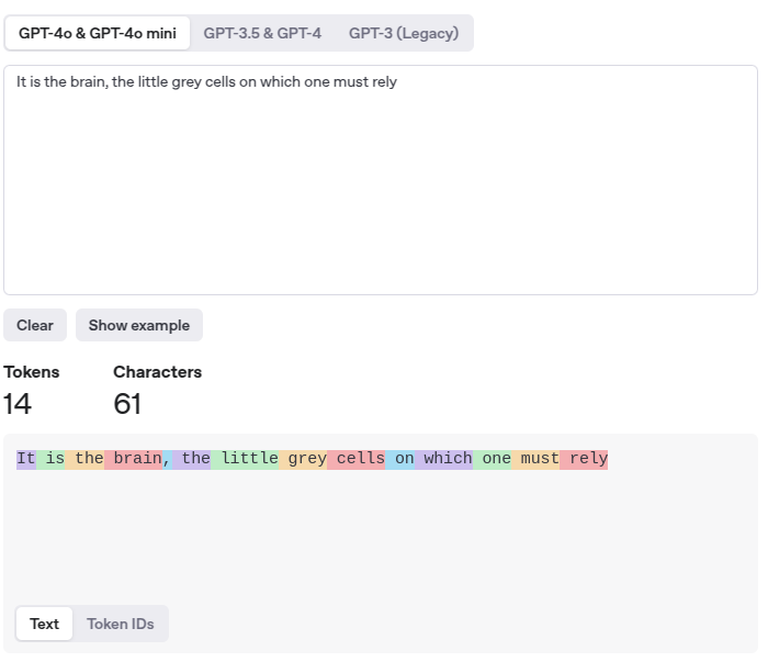
We obtain 14 tokens. In that case, every word corresponds to its own token, but that isn’t always true.
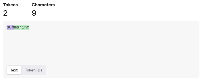
For instance, when we try the word 'submarine', it consists of two tokens. Since 'sub-' is a prefix that appears in many words, it is more efficient to define a specific token in our vocabulary.
In our case, we are interested in predicting letters, so we are not going to use OpenAI, but a custom one. Our vocabulary comprises the distinct characters required for our input —present in "It is the brain, the little grey cells on which one must rely" - :
We will need 17 tokens [a, b, c, e, g, h, i, l, m, n, o, r, s, t, u, w, y].
Alternatively, instead of predicting the next letter, we could have chosen to predict the next token —similar to modern language models such as BERT and GPT —which use words or subword units.
The embedding layer
Now that our vocabulary is defined, we need to represent it in a numeric format that the next layers understand. This process is known as embedding the tokens. I’ve already covered embeddings before, but let’s revisit the concept briefly. Each token in our vocabulary is linked to a vector in an n-dimensional space (an array of n values).
During the training phase, the model learns an embedding vector for each token by considering its context. It is important to note that we will not be using predefined embeddings here; instead, we will create our own embedding tailored to our specific content.
Let's take an example to be sure to understand. If we had decided to train a model using a general corpus like Wikipedia, the word “doctor” would be embedded in a vector space that links it to medicine, education, and healthcare. However, if we had decided to train the same model on a corpus of Agatha Christie novels, the word “doctor” would be embedded in a vector space related to crime, investigation, and mystery. It remains the same word “doctor,” but the meaning and relationships it has with other words differs because of the context.
During inference, we will simply use these learned embeddings and feed them into the next layer, which in this case will be our GRU layer (more on this later). Remember, embeddings capture semantic relationships, so similar concepts will have a smaller Euclidian distance than dissimilar ones. In this sense, the embedding layer serves as an “abstraction” layer: words that are “similar” in the context of our corpus will produce similar inputs for the subsequent layer.
The GRU layer
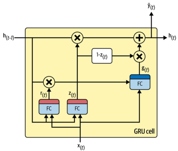
In this section, we examine the functioning of the GRU cell in schema 1. Although it might initially appear complex, we will break down the model systematically, step by step. By the end of the discussion, you will have a clear understanding of its mechanics.
Just as the embedding layer serves as the “abstraction” layer—allowing semantically similar concepts to be represented in like fashion—the GRU layer functions as the “memory” layer. It keeps track of previous tokens and uses this contextual information when processing new tokens.
Think of it as the brain of Poirot getting new information from it's witness: At each new word (input from the embedding layer) the brain asks: do I need to remember this? Should I forget what I was just thinking about? Should I update my memory with this new word?
We could represent the approach as two steps: Step 1—make a guess (candidate), and Step 2—decide how much of the guess to keep.
Step 1: Make a guess (candidate)
“If I reset part of my memory and mix it with this new input, what would a new state look like?”
Step 2: Decide how much of the guess to keep
“Should I actually use that guess? Or should I keep some (or all) of my old memory?”
Keep in mind, that the input consists of a vector containing the embedding for a token and that two embeddings with a small euclidean distance are considered semantically similar. When we change the value of a dimension—either by scaling it or altering it in any other way—we modify the semantic meaning associated with that dimension. Since embeddings typically range from -1 to +1, multiplying an embedding by a negative number (such as -1) will invert its meaning, while operations such as addition, subtraction, or scaling will modify its intensity—either softening or amplifying it. Multiplying by zero effectively “erases” the information contained in that dimension, resulting in a loss of information. For instance, consider a dimension that measures the sentiment of a token. A value of 1 indicates positive sentiment, –1 indicates negative sentiment, and 0 represents neutrality
We will start by analyzing the cell’s inputs and outputs independently of its content, thereby simplifying our approach..
We will start from the bottom and work our way up. The starting point in the GRU of schema X is the X(t) at the bottom, which is is simply the input vector for the tᵗʰ token produced by the previous embedding layer. Remember that each token has been embedded into a vector of n dimensions, meaning that the input vector contains n values at each step. All the tokens in our sequence will be transmitted sequentially to the GRU, which will produce an output for each token. This output will be used by the next layer to generate a result, which will then be compared with the character at the corresponding index in the target sequence.
The GRU’s output at each time step is context-dependent. This means each prediction is informed not only by the current token’s representation but also by the accumulated history encoded in the hidden state
Each output from the GRU will then consumed by the following (dense) layer, which will output the model's view of the next most probable token in our vocabulary (more on this later).
Now, let’s focus on the other direction by going from left to right. Here, the GRU takes the previous state (called the hidden state) as input h(t−1) and generates the next state h(t). This state, functioning as the cell’s memory, is then passed onward from one step to the next. As we saw earlier, the GRU output is context-dependent: because it has been influenced by all preceding inputs, the state enables the cell to analyze the current token within the context of earlier tokens. Note that the output of the GRU and its output state are the same value, simply routed to different targets.
Finally, let's examine how the input and the states combine to produce the output. Recall our two steps: first, determining what the new state should look like; and second, deciding whether to retain some of the old memory or replace it entirely ? It's time to see how these operations function are implemented in our GRU.
R(t) : the reset gate
To propose a new state (make a guess), we first employ the reset gate (R(t)). This gate combines the previous hidden state and the current input to produce an output array with values between 0 and 1. Each element of this array is then multiplied by the corresponding element in the previous hidden state.
This scaled state is then combined with the current input within the function G(x) to generate a candidate state
Recall that the input consists of an array of embeddings, where two embeddings with a small euclidean distance are considered semantically similar ? If the hidden state has been multiplied by 0 in the reset gate, the portion of the past in the candidate state becomes null, effectively "forgetting" it; conversely, multiplying it by 1 leaves it unchanged prior to be scaled and combined.
Finally, the cell can observe what the new state looks like. But it still has to decide whether to use that guess using the second gate : the forget gate.
Z(t) : the forget gate
The Z(t), or forget gate, is very simple. It decides how much of the previous hidden state to keep and how much of the new candidate state to add. To achieve this, the gate uses the current input along with the past hidden state to compute a factor. Then, it scales each state separately: the past state is multiplied by this factor, while the candidate state is multiplied by one minus the factor. Finally, the results are summed to produce the output.
The dense layer
The internals of this layer are straightforward. It has one cell for each vocabulary token: 17 in our case. When it receives a state from the GRU, each cell outputs the probability that its token will be the next character.
However, depending on the size of the vocabulary, this process can be very time-consuming. Some optimization techniques exist to avoid calculating the probability for every token, although we will not detail them here.
A few words on temperature
We could choose to simply always select the token with the highest probability. However, we can also allow the user to control the model's "creativity" by randomly choosing the next token based on its probability. For example, a token with a 20% chance of being selected may indeed appear 20% of the time.
The temperature parameter scales the token probabilities so that a higher temperature flattens the distribution—giving lower-probability tokens a better chance of being selected—while a lower temperature sharpens it, making the highest-probability tokens even more likely.
Et voilà, mon ami! You should now have a clear understanding of the internals of an RNN. From here, you can move on and start exploring the attention mechanism which is next topic on the road to llms